The Zero-Shot Plateau

My last post made a narrow claim: on a classification taxonomy of my own, a fine-tuned encoder beats the zero-shot “decision models” everyone shipped this autumn by about 30 macro-F1 points, at a fraction of the cost. Four fair objections came up, all some version of “you went easy on the zero-shot side”:

• Use a bigger or better zero-shot model.
• Fine-tune the decision model, then.
• Escalate the hard cases to a frontier LLM.
• Route on the confidence scores instead of taking the top label.

So I ran all four on the same dataset split. The short spoiler: two of the four roads dead-end on the same plateau, one works but mostly proves the labels were the point all along, and the last one works.

Same disclosure as before: my dataset, my label mapping, my class descriptions. Every number shares the same seeded stratified split (1,232 test items), body-only input, macro-F1.

“Use a bigger zero-shot model”

The obvious gap in the first post was that I never tried a general-purpose LLM. So I added Claude Haiku 5.5, which Anthropic had just repriced to $0.10 per million input tokens and markets for exactly this: high-volume classification and routing. Gave it the same five label descriptions every decision model got, without examples.

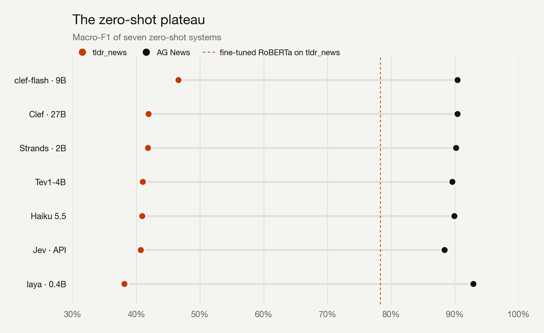
It scored 0.409, right in the middle of the decision-model pack. Here is the whole zero-shot field now: seven systems, five of them ranging from 0.4B to 27B parameters and two that don’t disclose a size.

System	Params	tldr_news (custom)	AG News (benchmark)
laya	0.4B	0.381	0.929
Jev (API)	undisclosed	0.407	0.884
Haiku 5.5	generalist	0.409	0.899
Tev1-4B	≈5B	0.410	0.896
Strands Decider	2B	0.418	0.902
Clef	27B	0.419	0.904
clef-flash	9B	0.466	0.904

From a 0.4B router to a 27B joint-head model to a general-purpose LLM, every zero-shot approach lands between 0.38 and 0.47 on my tldr_news taxonomy and jumps to 0.88-0.93 on AG News. A fine-tuned RoBERTa sits at 0.78 on the same split, 30 to 40 points above the entire field, for seven cents of training.

The ceiling is informational: a one-line description like “Business & Strategy: company news, markets, funding rounds” pins down maybe 40% of my editorial calls. The rest lives in conventions that exist only in my labels. No count of parameters recovers information that was never in the prompt. Putting labeled examples in the prompt lifts it about ten points at best, still far short of a fine-tune¹. Cloudflare’s distilled 9B clef-flash is the mild exception at 0.47, and it still sits over 30 points under RoBERTa. The odd part is that it beats its own 27B teacher off-distribution². My best guess is that the bigger model memorized the training mixture harder, which helps on AG News and hurts on mine.

“Fine-tune the decision model, then”

It was kind of expected that a fine-tuned decider beats a zero-shot one. The question worth testing is whether the decision-model architecture (the non-autoregressive head, the calibration training) buys anything over a plain encoder once you’ve spent the labels. So I LoRA-fine-tuned Tev1-4B, same prompt format as its zero-shot run, and put it on the label-efficiency curve next to the encoders.

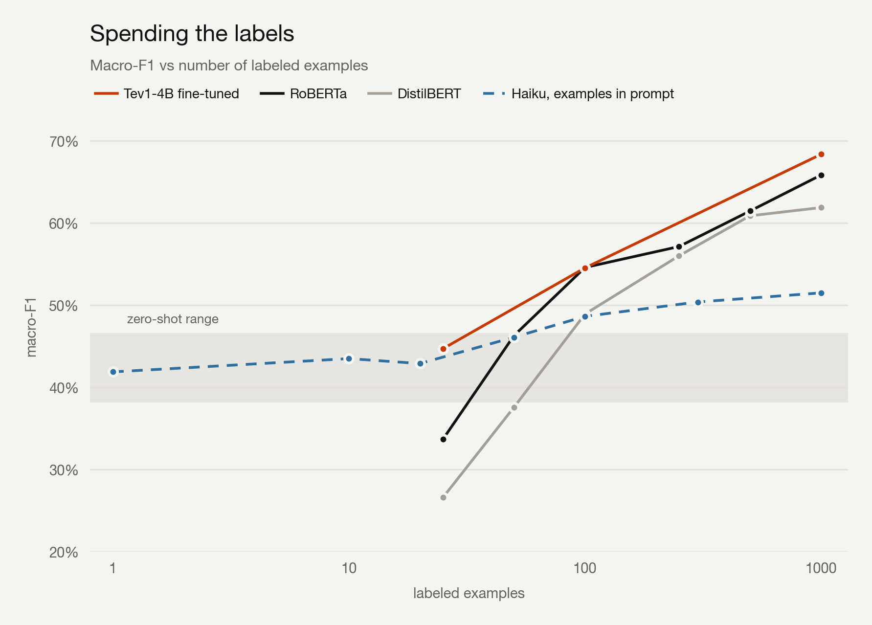
The answer has two halves. The 4B’s pretrained prior is a real head start: at 25 labels it reaches 0.45 while DistilBERT is still at 0.27, because a big model generalizes from a handful of examples where a small one is out of its depth. So if you have twenty-five labels and an afternoon, the fine-tuned decider is your best option.

But by 100 labels RoBERTa has drawn level, 0.55 to 0.55, and from there the two curves climb together: the 4B keeps a lead of about two points at 1,000 labels and at full data (0.80 vs 0.78), a margin about the size of the seed-to-seed variance on these curves, for a model that costs seventeen times as much per inference³. Its one lasting edge is calibration: it comes out of fine-tuning at ECE 0.036 with no post-hoc scaling, which the encoders need a temperature fit to match. So “fine-tune the decider” works. Past about a hundred labels, though, you’re paying 4B inference for encoder accuracy.

The dashed line in the chart is the third way to spend the same labels: hand them to Haiku as in-context exemplars instead of gradients. It follows the zero-shot band until about 50 examples, reaches 0.49 at 100, then flattens. A thousand exemplars, about 146k tokens of prompt, get it to 0.51, where the same thousand labels fine-tune Tev to 0.68 and RoBERTa to 0.66. And every single call re-reads all thousand¹.

“Escalate the hard cases”

Now the pattern of the season: let a cheap model answer what it’s sure of and route the rest to a big one. It’s the idea behind every cascade-routing stack shipping right now⁴, and the idea has deep roots. Confidence-based cascading was everywhere in the BERT era: TangoBERT routed between a small and a large BERT on exactly this signal, CascadeBERT stacked calibrated models, and the early-exit line (FastBERT, DeeBERT, my own early-exiting series) did the same trick across layers instead of across models. The modern router just puts a decision model in front. All of it rests on one assumption the plateau quietly breaks: that the thing you escalate to is better than the thing you have.

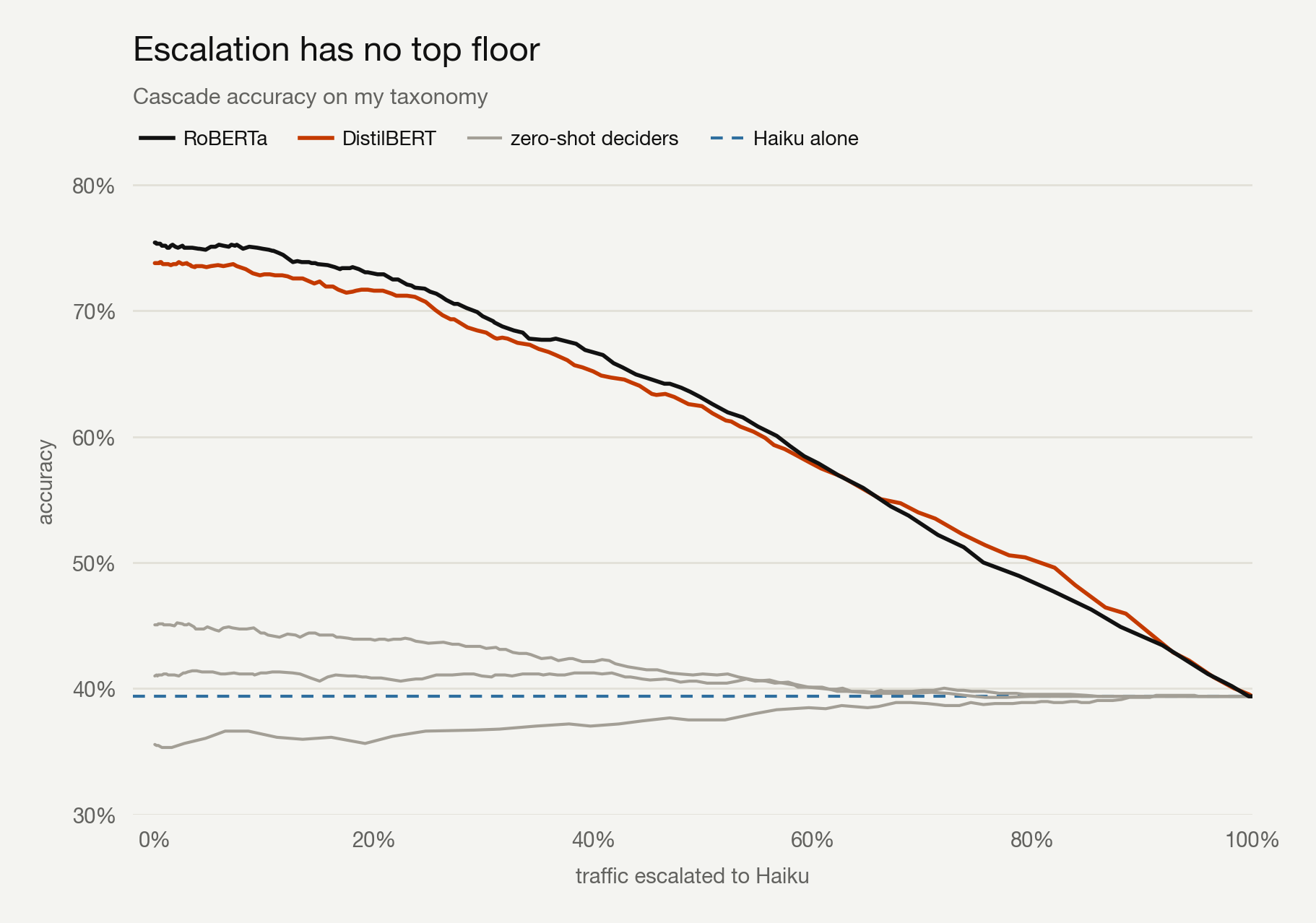
I simulated every cascade offline. Each first stage answers when its top label probability clears a threshold and escalates everything below it to Haiku, and I swept that threshold across its whole range. Two shapes come out.

Start with a zero-shot decider in front, the day-one setup. Escalation buys nothing here. Tev and Clef gain at most 0.4 points at any threshold, and laya only “gains” 3.9 points by escalating 91% of its traffic, which amounts to handing the whole stream to Haiku. The model you escalate to sits on the same plateau, so there’s nothing above you to reach.

Put a fine-tune in front instead and escalation actively hurts. The fine-tune is right 75% of the time, Haiku 39%, and even on the low-confidence items the fine-tune hands off, it still beats Haiku. Every escalation swaps a better answer for a worse one, so the cascade slides from 0.75 toward 0.39 as you escalate more.

The decline itself is unsurprising. The interesting part is why confidence can’t rescue it. The errors do decorrelate: an oracle that escalated exactly the fine-tune’s mistakes would reach 0.84, because Haiku rescues about a third of them. But the items the fine-tune is unsure about are mostly the items Haiku gets wrong too, the truly ambiguous ones that no second opinion resolves, so the confidence signal escalates the wrong examples. And it escalates them expensively: every call up to Haiku is roughly $85 per million on top of the fine-tune’s $1.58, spent to move accuracy backwards. The oracle gap is real, and confidence routing can’t reach it. That’s the cascade’s hidden dependency: it only works when something above you knows your labels. In-distribution something does, which is why the pattern works on benchmark-shaped tasks, and why it worked across the layers of the BERT cascades, where every exit trained on the same data. On your taxonomy, nothing does until you teach it.

“Route on the confidence scores”

The last objection is the one that works, and it’s worth slowing down on, because the instinct is right. Routing on confidence is exactly what you should do. The twist is the destination: you route the uncertain items to a human, not a bigger model. And whether that pays off depends on a property you can measure: does the model know what it doesn’t know?

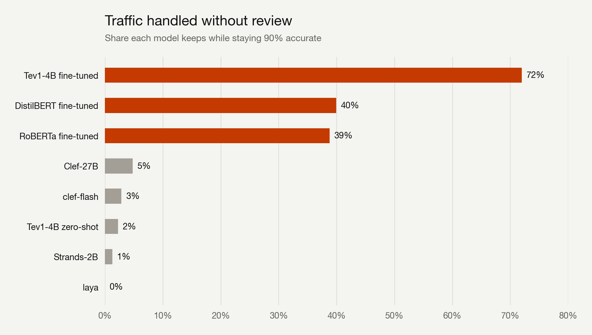
Sort each model’s predictions by confidence and ask how much traffic it can keep for itself while staying at least 90% accurate on what it keeps, sending the rest to review. To keep it honest, each model’s confidence threshold is picked on a held-out validation half and then applied, frozen, to the test set. The fine-tuned models carry between a third and nearly three quarters of the stream, and their thresholds transfer: kept-item accuracy lands within about a point of the bar. The zero-shot decision models, whose signature feature is calibrated confidence, keep under 5%, and apart from clef-flash even that sliver misses the promise, coming back 69-73% accurate on the items they chose to keep.

The cleanest version of the result is the same model twice. Zero-shot, Tev1-4B keeps 2% of traffic and is only 71% accurate even on that slice. Fine-tuned on my labels, the identical architecture keeps 72% and holds the bar. The deciders’ calibration machinery is good (Clef’s Brier training is excellent in-distribution), but calibration leaves the training distribution no better than accuracy does. Across the full confidence range the fine-tunes score an area under the risk-coverage curve of 0.07 to 0.14, against 0.44 to 0.57 for the zero-shot field⁵. On top of being more accurate, the fine-tune is a three-to-eight-times better judge of its own limits, which is the property a router actually runs on.

The intuition: a probability is only as trustworthy as the model’s sense of where the decision boundary lies. Fine-tuning on in-domain labels is what draws that boundary in the right place, so the model’s confidence starts tracking its correctness on your data, and high confidence really does mean likely-right. A zero-shot model is sure about a boundary it learned from someone else’s distribution, so on your taxonomy its confidence ranks examples by the wrong thing and no threshold cleanly separates the predictions worth keeping. That is why the same Tev is useless as a router at zero-shot and dependable once fine-tuned: the labels are what make its confidence mean something here.

Where each approach fits

The previous post’s conclusion holds, and this one fills in the details. Zero-shot decision models, and Haiku 5.5 alongside them, are the right call on day one: no labels, a taxonomy still in motion, many small tasks behind one endpoint, and anything close to a benchmark distribution, where they’re fast, cheap, and honestly calibrated.

The moment the taxonomy is yours, every road runs through labels. Twenty-five of them and a fine-tuned 4B decider is the best start you can buy. A hundred and a fine-tuned encoder matches anything in the field at a fraction of the cost. And the labels are not optional even if you stay zero-shot, because the only way to know whether any of this works on your data is a labeled eval set, at which point a fine-tune costs seven cents more than the measurement you were already paying for, and it’s the only option that also knows when to ask for help.

The obvious caveat is that this is one dataset: five classes, my labels, my class descriptions. Better-written descriptions might move the zero-shot field a few points, and a taxonomy closer to news-desk categories would move it a lot, as AG News shows. What I’d bet on is the shape: zero-shot scores track how far your labels sit from what the model saw in pretraining, and only labels close that distance. The cheapest way to prove me wrong is to run the same four roads on your own data.

---

Reproducibility. Same harness as the previous post. Encoders fine-tuned with bert-squeeze on a Modal L4, laya and Tev zero-shot on L4/T4, Clef and clef-flash from their open weights on an H100, Strands Decider from its package on an L4, the Tev LoRA fine-tune and sweep on an H100, and Haiku 5.5 via the Batch API with a structured-output label enum, except the many-shot sweep, which ran through the Nous Portal gateway (same model, synchronous API) after the batch workspace hit its monthly spend limit. The cascade and coverage numbers are offline computations over per-item probability dumps, aligned across models by text hash. Those dumps come from the calibration-protocol reruns, whose prompts differ cosmetically from the headline runs, so per-model accuracy there can sit a point or two away from the table’s macro-F1. Dataset: tldr_news, five content classes, body-only input.

1. Haiku takes exemplars where the frozen deciders can’t, so I swept them: 1, 10, 20, 50, 100, 300 and 1,000 stratified in-context exemplars score 0.419, 0.435, 0.429, 0.461, 0.486, 0.504 and 0.515. The climb is real up to about a hundred, then it flattens. At 1,000 examples Haiku sits 17 points under the Tev fine-tune and 14 under RoBERTa on the same labels, and carries ~146k exemplar tokens into every call: roughly $15,000 per million classifications at list price, still ~$1,500 with prompt caching, against $1.58 for the better model. ↩ ↩²

2. clef-flash 0.466 vs Clef 0.419 on my taxonomy, and it’s 2.2× faster (152 ms vs 341 ms, batch 1 on an H100). ↩

3. About $27 vs $1.58 per million classifications, from the cost model in the previous post. ↩

4. For example vLLM-SR’s “decision models need a router”, which cascades a small decider into a large one on low confidence. ↩

5. Area under the risk-coverage curve, lower is better. Fine-tuned Tev 0.07, RoBERTa 0.12, DistilBERT 0.14. Clef and clef-flash 0.44, Strands 0.44, Tev zero-shot 0.50, laya 0.57. ↩