DeeBERT: Teaching BERT When to Stop Thinking
Why does BERT need twelve layers to classify “I love this movie” as positive?
In 2020, Microsoft researchers watched their models burn through millions of Transformer operations on queries a third-grader could handle. Every input—from “dogs are animals” to complex medical diagnosis—consumed identical computational resources. The waste was staggering.
DeeBERT changed that. It introduced the first practical early exiting system for Transformers, proving that models could learn not just what to predict, but when they knew enough to stop predicting.
The Highway Architecture
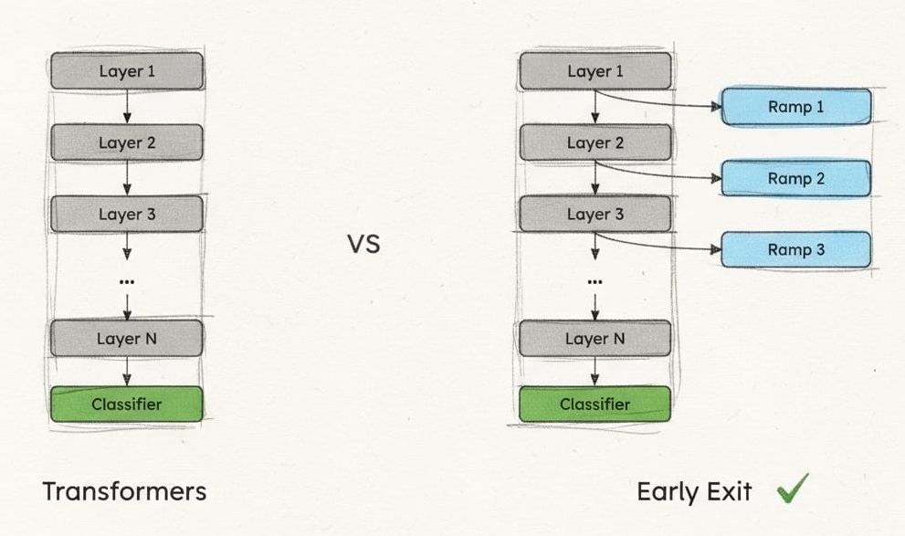
DeeBERT’s insight was architectural simplicity. Don’t redesign BERT. Add exit ramps.
The intuition came from highways. Not every car needs to drive the full route—some destinations are closer than others. Why force every input through twelve Transformer layers when some might resolve their “destination” (classification) after just three or four layers? The challenge was making these exits lightweight enough that they didn’t slow down traffic for inputs that needed the full journey.
Each transformer layer gets an “off-ramp”—a tiny classification head that can make predictions from that layer’s representations. The genius is in what these off-ramps don’t include: no additional transformer blocks, no complex attention mechanisms, no heavyweight processing. Just the minimum viable predictor.
class HighwayExit(nn.Module):
    def __init__(self, hidden_size, num_classes, p_dropout):
        super().__init__()
        self.pooler = nn.Linear(hidden_size, hidden_size)
        self.dropout = nn.Dropout(p_dropout)
        self.classifier = nn.Linear(hidden_size, num_classes)

    def forward(self, hidden_states):
        pooled = self.pooler(hidden_states[:, 0])  # [CLS] token
        pooled = nn.Tanh()(pooled)
        pooled = self.dropout(pooled)
        return self.classifier(pooled)
The pooler serves a specific purpose: it transforms the [CLS] token representation into a format optimized for
classification. The tanh activation provides bounded outputs, preventing extreme values that could destabilize early
predictions. Dropout remains critical—without it, early exits overfit catastrophically to their limited view of the
data.
The parameter overhead reveals the elegance. For BERT-base with 768-dimensional hidden states, each off-ramp adds
approximately 768 × 768 (pooler) + 768 × num_classes (classifier) parameters. Across twelve layers with binary
classification, that’s roughly 7.4M parameters total—just 6.7% overhead on BERT-base’s 110M parameters. You get twelve
potential exit points for the cost of a single additional layer.
The architecture transforms the computational contract:
This isn’t just an optimization. It’s a fundamental shift from “process to depth N” to “process until confident.” The model learns not just to transform inputs, but to recognize when those transformations are sufficient.
The Training Trap
Jointly training the model backbone and the added “off-ramps” fails badly, and understanding why reveals deep insights about neural network optimization.
Imagine teaching twelve students where each must learn the same material but can only see a progressively clearer picture. Student 1 sees a blurry image, Student 2 sees it slightly clearer, and so on. If you test all students simultaneously and average their grades, what happens? The early students drag down the average, so you naturally focus on helping them. But when you do, the advanced students—who could achieve perfect scores with the clear picture—start failing because the teaching pivots to accommodate the struggling early students.
This is exactly what happens with joint training of multiple exits. The loss landscape becomes:
\[L_{\text{joint}} = \sum_{i=1}^{12} w_i \cdot L_i\]Setting the weights $w_i$ creates an impossible optimization problem. Favor early layers with high weights, and the model learns representations that work well for shallow prediction but fail at depth. Favor late layers, and early exits never learn to extract useful signals from partial information. The gradients fight each other, creating a compromise that satisfies no one.
DeeBERT’s solution was conservative but brilliant: two-stage training that separates the competing objectives.
# Stage 1: Build foundation (standard BERT fine-tuning)
for epoch in range(num_epochs_stage1):
    for batch in train_loader:
        hidden_states = model.bert(batch.input_ids)
        loss = criterion(model.classifier(hidden_states[-1]), batch.labels)
        loss.backward()
        optimizer.step()

# Stage 2: Specialize exits (frozen backbone)
model.bert.requires_grad_(False)
model.classifier.requires_grad_(False)

for epoch in range(num_epochs_stage2):
    for batch in train_loader:
        hidden_states = model.bert(batch.input_ids, output_hidden_states=True)
        losses = []
        for i in range(11):  # Train only intermediate exits
            logits = model.exits[i](hidden_states[i])
            losses.append(criterion(logits, batch.labels))
        total_loss = sum(losses) / len(losses)
        total_loss.backward()
        optimizer_exits.step()
Stage 1 ensures the highway is perfectly built, meaning, the transformer learns optimal representations for the full journey. Stage 2 then asks: “Given this fixed highway, where can we add useful exits?” The frozen backbone provides stable features, preventing the exits from corrupting each other’s learning.
The paper states the reasoning explicitly: “The reason for freezing parameters of transformer layers is to keep the optimal output quality for the last off-ramp.” This isn’t just about preserving quality. It’s about admitting that optimizing for multiple depths simultaneously might be impossible with current methods.
The trade-off is subtle but important. Those intermediate classifiers must work with representations optimized for 12-layer processing, not early prediction. It’s like asking someone to solve a puzzle with pieces designed for a different puzzle—possible, but suboptimal.
Entropy as Confidence
DeeBERT needed a way for the model to express uncertainty, to say “I don’t know enough yet.” The proposed solution came from information theory: entropy.
Think about rolling dice. A fair die has maximum entropy: all outcomes equally likely. A weighted die that always lands on 6 has zero entropy—no uncertainty. For neural nets, the probability distribution over classes behaves similarly. When the model assigns 95% probability to one class and spreads 5% across others, it’s like a heavily weighted die—low entropy, high confidence. When probabilities are evenly distributed, it’s like a fair die—high entropy, maximum uncertainty.
\[H = -\sum_{i} p_i \log(p_i)\]The logarithm serves a specific purpose: it makes the measure additive across independent events and penalizes uncertainty non-linearly. Being 50-50 between two choices is much worse than being 90-10, which the log captures mathematically.
def compute_entropy(logits):
    probs = F.softmax(logits, dim=-1)
    log_probs = torch.log(probs + 1e-8)  # Numerical stability
    entropy = -torch.sum(probs * log_probs, dim=-1)
    return entropy

def normalized_entropy(logits, num_classes):
    """Normalize to [0, 1] for comparison across different class counts"""
    entropy = compute_entropy(logits)
    max_entropy = torch.log(torch.tensor(num_classes))
    return entropy / max_entropy
The numerical stability term (1e-8) prevents log(0) errors when the model is extremely confident. Normalization matters because raw entropy isn’t comparable across tasks—binary classification has maximum entropy of log(2) ≈ 0.69, while 10-class classification peaks at log(10) ≈ 2.30.
During inference, the decision process becomes algorithmic:
def forward_with_early_exit(model, inputs, entropy_threshold):
    hidden = model.embeddings(inputs)
    for i, (layer, exit) in enumerate(zip(model.layers, model.exits)):
        hidden = layer(hidden)
        logits = exit(hidden)
        if compute_entropy(logits) < entropy_threshold:
            return logits, i  # Exit at layer i
    return logits, 11  # Didn't exit early
The threshold becomes your control knob. Set it to 0.1 and only the most confident predictions exit early—you prioritize accuracy over speed. Set it to 0.5 and more samples exit early—you trade accuracy for efficiency. The relationship isn’t linear: the first 0.1 increase might barely affect accuracy, while the next 0.1 could cause significant degradation.
The elegance hides a fundamental flaw: neural networks are overconfident by nature. They’ll output 99% confidence while being completely wrong, especially on out-of-distribution inputs. Entropy measures how peaked the distribution is, not whether that peak points to the correct answer. This limitation would spark intense research into better confidence estimation.
What BERT Revealed
DeeBERT didn’t just accelerate inference, it became a diagnostic tool for understanding transformer learning dynamics.
The first surprise was that BERT and RoBERTa learn fundamentally differently. BERT builds understanding incrementally—each layer adds a bit more accuracy, a bit more nuance, steadily climbing toward final performance. RoBERTa does something stranger. Early layers accomplish almost nothing, sometimes even hurting accuracy. Then suddenly, around layer 4 or 5, performance jumps dramatically. Another plateau, then another jump.
This matters because it reveals that the path to the right answer isn’t universal. Different architectures, different pre-training objectives, different data—they all create models that think differently about the same problems. You can’t assume that layer 6 means the same thing in BERT as in RoBERTa.
The second revelation was systematic redundancy. Watch how samples distribute across exit layers and a pattern emerges: certain layers become popular exits while others are nearly abandoned. The abandoned layers are precisely those that add minimal quality improvement.
Even more striking: the final layers in BERT-large and RoBERTa-large often degrade performance. These models carry their last 15-20% of parameters as dead weight, contributing nothing or even hurting results on many tasks. We’d been scaling models up without questioning whether all that depth was necessary.
The third insight was that samples naturally cluster by complexity. Simple sentiment like “I love it” exits at layer 3. Straightforward negations like “I didn’t love it” might need layer 5. Complex adversative constructions like “The acting was stellar, though the plot felt disjointed” require the full depth. The model learns to route inputs appropriately without explicit supervision—just by trying to minimize both task loss and entropy thresholds.
This self-organization reveals something profound about neural networks: they’re not just learning to solve tasks, they’re learning representations of task difficulty. The same mechanism that learns to classify sentiment also learns to recognize which sentiments are hard to classify. That meta-knowledge was always there, latent in the model. Early exit just made it explicit and useful.
The pain point these revelations expose: we’ve been wasting massive amounts of computation by treating all inputs uniformly. Every query burns through all layers regardless of necessity. Every simple case pays the cost optimized for complex cases. The efficiency loss isn’t a minor optimization opportunity—it’s a fundamental architectural mismatch between how we build models and how they should actually run.
The Batching Problem
DeeBERT’s Achilles’ heel emerged in production: batch processing breaks completely.
Modern deep learning relies on batching for efficiency. A GPU processing 32 samples simultaneously achieves 10-20× higher throughput than processing them sequentially. The hardware is designed for it—tensor cores operate on matrices, memory bandwidth gets amortized, kernel launch overhead disappears. Breaking this paradigm hurts.
The breaking point is simple:
if highway_entropy < self.early_exit_entropy[i]:
    highway_logits_all = highway_logits
    # ... exit logic
This conditional works for single samples. For batches, PyTorch throws:
RuntimeError: Boolean value of Tensor with more than one value is ambiguous
In a batch of 32 samples, maybe 10 want to exit at layer 3, 15 at layer 7, and 7 need all 12 layers. How do you handle this? Every solution has major drawbacks.
Padding everyone to the maximum depth defeats the entire purpose. Processing samples individually throws away GPU efficiency. Dynamically regrouping samples as they exit requires complex bookkeeping and memory management that current frameworks don’t support.
The fundamental issue is architectural. GPUs achieve peak efficiency through uniform computation—every thread in a warp executing identical instructions. Mix different computation paths and efficiency plummets. It’s like a highway where some cars can teleport but only if all cars in their lane teleport to the same exit. The constraint seems absurd but reflects how our hardware actually works.
The Classification Ceiling
DeeBERT’s deepest limitation wasn’t architectural—it was conceptual. The system needs discrete probabilities to compute entropy. No probabilities, no confidence measure, no early exit.
This seems like a minor detail until you consider what it excludes. Regression tasks predict continuous values—how do you compute entropy over infinite possibilities? Generation tasks select from 50,000-token vocabularies—technically discrete, but entropy becomes meaningless when spread across so many options. Span extraction tasks predict start and end positions—two separate distributions that need joint consideration.
The limitation reflects a deeper assumption: that confidence can be reduced to a single scalar. For classification, this works. The model predicts one of N classes, uncertainty naturally maps to entropy. But most modern NLP transcends classification.
Consider text generation. At each position, the model might be confident about avoiding certain tokens (definitely not “ purple” after “The sky is”) while uncertain about the exact choice (“blue” vs “cloudy” vs “clear”). Traditional entropy captures neither the partial certainty nor the nature of the uncertainty.
The field’s response was to abandon task-specific confidence entirely. BERxiT introduced learnable exit predictors that directly answer “should I continue?” rather than deriving it from task predictions:
class LearnedExitPredictor(nn.Module):
    def __init__(self, hidden_size):
        super().__init__()
        self.exit_head = nn.Linear(hidden_size, 1)

    def forward(self, hidden_states):
        # Predict "should I continue?" directly
        continue_score = torch.sigmoid(self.exit_head(hidden_states[:, 0]))
        return continue_score
This decouples early exit from task-specific confidence, enabling any task type. But it creates a new problem: how do you train this exit predictor? What signal tells it when to exit? The solution requires careful data collection—tracking which samples succeed at which depths—or sophisticated training objectives that balance efficiency and accuracy.
The classification ceiling revealed early exit’s fundamental challenge: the “when to stop” decision might be harder than the task itself. DeeBERT solved it for one narrow case. Generalizing that solution remains an open problem.
References
You can find a full DeeBERT implementation using Lightning on my bert-squeeze repository.
[1] - BERT: Pre-training of Deep Bidirectional Transformers for Language Understanding
[2] - DeeBERT: Dynamic Early Exiting for Accelerating BERT Inference
[3] - RoBERTa: A Robustly Optimized BERT Pretraining Approach
Next: How entropy-based confidence became both DeeBERT’s breakthrough and its Achilles’ heel. We’ll implement BERxiT’s learned exits, and trace how fundamentally different philosophies emerged for the “when to exit” problem.